Probabilistic Forecasting: How to Read Timestral’s 21 Quantiles

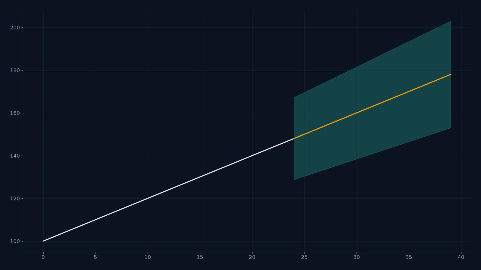
A point forecast says “demand will be 100.” A probabilistic forecast says “demand will be between 70 and 140, with a median of 100.” The second sentence is more useful for almost every real decision, because the cost of being wrong is asymmetric: running out of stock is not the same as holding one extra unit.

Timestral returns 21 quantiles per forecast step. This guide explains what they are, how to read them, and how to use them without turning every decision into a statistics project.

CSV forecast studio

Paste a series, get a probabilistic forecast.

One value per row, or a date column plus one or more numeric columns. Timestral returns a median forecast and a likely range. The demo runs on the public Hugging Face Space; the API is the paid product.

1 · Paste or upload a CSV2 · Pick a horizon3 · Download the 21 quantiles

Upload CSV

Steps

Airline passengersMonthly salesWebsite visitsElectricity load

month,passengers 1949-01-01,112 1949-02-01,118 1949-03-01,132 1949-04-01,129 1949-05-01,121 1949-06-01,135 1949-07-01,148 1949-08-01,148 1949-09-01,136 1949-10-01,119 1949-11-01,104 1949-12-01,118 1950-01-01,115 1950-02-01,126 1950-03-01,141 1950-04-01,135 1950-05-01,125 1950-06-01,149 1950-07-01,170 1950-08-01,170 1950-09-01,158 1950-10-01,133 1950-11-01,114 1950-12-01,140 1951-01-01,145 1951-02-01,150 1951-03-01,178 1951-04-01,163 1951-05-01,172 1951-06-01,178 1951-07-01,199 1951-08-01,199 1951-09-01,184 1951-10-01,162 1951-11-01,146 1951-12-01,166

↗Run forecast1 credit per API call · the web demo is free while the public Space is available

Quantiles in one minute

A quantile is a cut point in a distribution. The 0.1 quantile is the value that the outcome falls below 10% of the time. The 0.5 quantile is the median. The 0.9 quantile is the value the outcome falls below 90% of the time.

The interval between the 0.1 and 0.9 quantiles is an 80% prediction interval: if the model is calibrated, roughly 80% of future outcomes should land inside it.

Timestral returns 21 quantiles, from the lower tail to the upper tail. The exact levels are part of the model; the studio shows a median and an 80% band by default. The CSV contains all 21, so you can choose a different band for your own decisions.

Why 21 and not 3

Three numbers (low, median, high) are enough for a dashboard. They are not enough for optimization. If you are choosing an inventory level, a staffing plan or a battery dispatch, you need to evaluate the cost of each possible outcome. More quantiles give you a finer approximation of the distribution.

The 21 quantiles also let you measure calibration at several levels. You can check whether the 50% interval contains about 50% of outcomes, the 80% interval about 80%, and the 98% interval about 98%. A model that is accurate at the median but wrong in the tails is dangerous for risk decisions.

The fan chart

A fan chart plots the quantiles as a widening band around the median. It communicates three things at once:

1. The central path — where the model thinks the series is going.
2. The uncertainty — how wide the band is.
3. The shape of the uncertainty — whether the band widens smoothly, jumps, or is asymmetric.

A band that widens slowly suggests a stable series. A band that explodes suggests high volatility or a horizon beyond the model’s useful range. A band that is asymmetric suggests the model expects more upside than downside, or vice versa.

Calibration is not accuracy

Accuracy asks “how close is the median?” Calibration asks “does the stated uncertainty match reality?” A model can be accurate on average and badly calibrated in the tails. For risk work, calibration matters more.

A simple calibration check:

1. Collect a backtest set of forecasts and actuals.
2. For each forecast, record whether the actual fell inside the 80% interval.
3. Average the indicator across many forecasts. It should be close to 0.8.

If the actual is inside the 80% band only 50% of the time, the model is overconfident. If it is inside 95% of the time, the band is too wide and you are paying for unnecessary safety stock.

Using quantiles for decisions

Inventory

If the cost of a stockout is high and the cost of holding is low, use a high quantile (for example, the 0.9) as the stocking target. If holding is expensive and stockouts are cheap, use a lower quantile.

Staffing

Use the median for the baseline schedule and the upper quantile for on-call capacity. The gap between them is the buffer you are buying.

Energy and capacity

Use the full distribution to evaluate dispatch or battery schedules. The tail quantiles are where the expensive events live.

Anomaly detection

A forecast band is a natural anomaly detector: if the actual leaves the 98% interval, something unusual happened. See time-series anomaly detection for the workflow.

What the band does not tell you

• It does not include model risk. If the world changes in a way the history has never seen, the band may be too narrow.
• It does not include causal effects. A price change or a new competitor is not in the model unless you encode it as a covariate.
• It is not a guarantee. Calibration is an empirical property; check it on your own backtest.

A practical workflow

1. Start with the median and the 80% band.
2. Backtest both the median error and the interval coverage.
3. If the band is too wide, shorten the horizon or reduce the series volatility (for example, aggregate to weekly).
4. If the band is too narrow, do not simply widen it by hand; check for missing covariates or a regime change.
5. Choose the quantile that matches your cost asymmetry.
6. Re-check calibration every month.

What to read next

• What is Timestral? — the model family.
• How to evaluate forecasts — MAE, RMSE, coverage and backtesting.
• Time-series anomaly detection — using the band as an alarm.
• API pricing — one credit per forecast call.

FAQ

What quantiles does Timestral return?

The model returns 21 quantiles per step. The studio shows a median and an 80% band by default; the CSV contains all 21.

Is the 80% band a confidence interval?

It is a prediction interval for the future outcome, not a confidence interval for a model parameter. The interpretation is “the outcome falls inside this range about 80% of the time,” assuming the model is calibrated.

Can I get a 95% band?

Yes. Use the 0.025 and 0.975 quantiles from the CSV, or select a wider band in the Space settings.

Why is the band wider at longer horizons?

Uncertainty compounds. A one-step forecast is usually tighter than a 36-step forecast. If the band explodes, the horizon may be beyond what the history supports.